Dissertation Study 3
Estimating the effect of demographic changes on participation in test boycotts
One study of my dissertation analyzes the causal impact of changing demographics within a school on student participation in boycotts of annual standardized tests. Based on research in social movements theory and educational policy, I hypothesize that when schools see increases in the share of students of color, students are more likely to participating in testing boycotts. This is called group threat. Basically, it predicts that members of majority groups will mobilize to take collective action when they are exposed to more members of minority groups.
My case is the opt-out movement–a coalition of parents and educators who oppose the use of standardized tests for school accountability purposes–what they call “high-stakes” tests. The movement emerged around 2010, but really picked up steam in 2013. By 2016, around 20% of students in New York, where the movement is the strongest, boycotted the annual tests.
Reasons for joining movements are multifaceted. People choose to join movements for ideological or personal reasons. I hypothesize that group threat played an important role, net of other factors.
To test this hypothesis, I use a panel of school-level accountability data from New York state. These data are publicly available from the Department of Education’s website. I supplemented these data with data from the Common Core of Data, which contains administrative and demographic data for every school in America.
I have already created my dataset. I use data from the 2008-2009 until the 2016-2017 school year. The dataset contains demographic data, testing data, and–most important of all–participation data. So for each school in New York, I have data on the number of student who participated, the average tests scores by grade, and the proficiency rates by grade. I will describe variables I use in a moment.
To identify the causal relationship between demographic changes and testing boycotts, I use a difference-in-differences framework, a common econometric technique for making causal inferences from observational data. There are several problems with observational data, in contrast with experimental data, when it comes to causal inference. In this case, maybe the school that experienced demographic changes were different from schools that did not experience those changes in critical ways related to test boycotts. Say, for example, that the parents of students of color were more likely to move their children to more schools where parents were highly educated. Well, more educated parents are more likely to have the time and resources to join social movements. So any relationship between demographic changes and testing boycotts would be spurious–the true cause would be parental education.
The difference-in-differences framework gets around this problem by netting out any pre-existing differences between the two groups of schools. How?
Image that we have an experiment. Schools in the experimental or treatment condition have an increase the share of students of color. The schools in the control group do not. The treatment is applied at a particular point in time (here, beginning in the 2012-2013 school year, the first year of meaningful participation in the boycott). In the experiment, with random assignment of schools to treatment and control conditions, we can simply find the mean difference in participation in the boycott and wham! We’ve estimated the causal impact of group threat.
Well with observational data, we don’t have the luxury. We have to accept that schools in the “treatment” group and the “control” group are different in many ways, some of which we can statistically control for, some of which (the more pernicious of which) we cannot because they are unobservd. But we can make a reasonable assumption–that, regardless of their differences, the schools in the two groups have parallel trends in the outcome measure in absence of the treatment. That is to say, while the schools have different levels of an outcome, the trends over time are the same. The application of the treatment for the treatment group changes the trend line for that group. This departure from the hypothetical trend is the causal effect of the treatment.
To do this is actually quite simple–find the difference in the outcome from time 0 to time t from the control group; find the differences in the outcome from time 0 to time t from the treatment group; and then find the difference between those differences. In a regression framework, it is a bit more than simply finding differences, since I will want to control for time-varying variables that I believe are correlated with boycotts of the tests.
Enough background, here’s the data.
Exploratory analysis
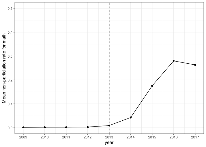
Prior to the 2012-2013 (from now on, I will refer to the school year by the year-end) school year, basically all students in New York took the annual standardized tests. These tests are mandatory and there are potential penalities for schools if students do not take them. For the most part, students did well on the test–about 70% proficiency rates overall. But beginning in 2013, the state adopted a new, more “rigorous”, assessment aligned with the recently developed Common Core State Standards. Proficiency rates dropped, helping to fuel the protest movement. No in this context, I hypothesize that group threat will increase testing boycotts. Without getting bogged down in sociological theory, the basic idea is that parents (particularly white parents) associate students of color with poor school performance and increased government regulation of schools. This threatens educational goods they feel entitled to–such as a rich diverse curriculum, extra-curricular activities, child-centered instruction. Research suggests that these goods are less likely found in schools that experience government regulation.
Note: For simplicity, I focus on the mathematics test. Students also take tests in reading and science. Note 2: I only use data from K-8 schools. The testing situation in high schools is much more complicated.
Starting in 2013, the proportion of students not participating in annual math testing increased, maxing out at about 20%.
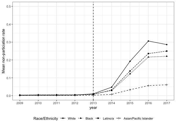
The students participating in the boycott are primarily, but not exclusively, white.
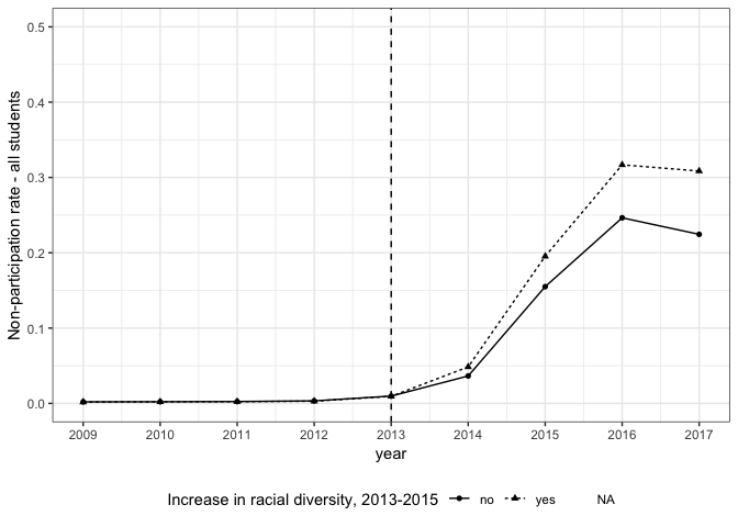
Schools that had increases in racial diversity between 2013 and 2013 had more students participating in the boycott than schools that did not–a bit of evidence for the group threat hypothesis.
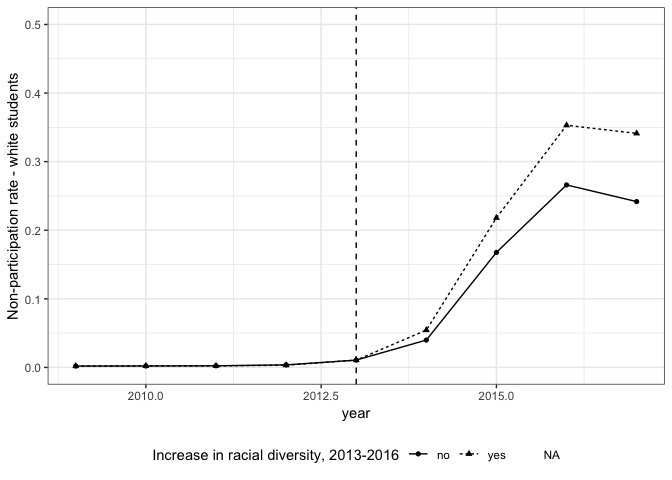
Again, we see this trend is true if we focus only on white students.
Difference-in-differences analysis
My main dependent variable is the proportion of students boycotting the annual math standardized test.
My main independent variable is the racial diversity of a school, captured using the Simpson diversity index common in ecological research. The index measures the population of each group in some setting–in this case, race/ethnicity groups within schools. My hypothesis is that schools that experience increases in racial diversity will have higher proportions of students boycotting the test. So schools with increases are in the “treatment” group. So I will create an indicator for schools that have a net increase in racial diversity during the treatment period–between 2013 and 2016. I have to choose a cutoff here–what increase is meaningful, according to this measure?
library(tidyverse)
ny_panel <-
  ny_panel %>%
  group_by(entity_cd) %>%
  mutate(change_per_black_hisp =
           round(per_black_hisp, 2) - round(dplyr::lag(per_black_hisp), 2),
         )

summary(ny_panel$change_per_black_hisp)
##    Min. 1st Qu.  Median    Mean 3rd Qu.    Max.    NA's
## -0.7200 -0.0100  0.0000  0.0039  0.0100  0.7100    2325
Now I will create an indicator for schools that had a net increase in the share of black and Latinx students between 2013 and 2015.
ny_panel <-
  ny_panel %>%
  mutate(
    increase_blhp_2013_2015 =
      ifelse(sum(change_per_black_hisp[year >= 2013 & year <= 2015], na.rm = T) > 0,
                  1, 0)
    )

table(ny_panel$increase_blhp_2013_2015)
##
##     0     1
##  8219 10418
To set up the difference-in-differences analysis, I need to create an indicator for the treatment period. This is the period after 2013. So for each school in the dataset, post2013 == 1 when the year is after 2013 and post2013 == 0 otherwise.
ny_panel <-
  ny_panel %>%
  mutate(post2013 = as.numeric(year > 2013))

table(ny_panel$year, ny_panel$post2013)
##
##           0    1
##   2009 2146    0
##   2010 2158    0
##   2011 2096    0
##   2012 2098    0
##   2013 2039    0
##   2014    0 2033
##   2015    0 2028
##   2016    0 2026
##   2017    0 2013
The difference-in-differences estimator is the interaction between post2013 and increase_diverse. This compares the proportion of students boycotting the test in schools that had an increase in diversity between 2013 and 2016 to those that did not and all schools before 2013.
Here’s the basic regression model:
[Y_{it} = \alpha_0 + \beta_1 R_i * D_t + \beta_2 R_i + \beta_3 D + \beta_4 X_{it} + \epsilon_{it}]
where (Y_{it}) is the proportion of students boycotting the test in school (i) in year (t), (D_t) is the indicator for years after 2013, and (R_i) is the indicator for the increases in racial diversity for school (i). (X_{it}) is a vector of relevant time-varying covariates and (\epsilon_{it}) is a school-year stochastic error term.
Since we have panel data, we can exploit within-school changes in order to control for any fixed unobserved differences between schools. This does a lot to help me aviod omitted variables bias, a constant threat to causal inference. Schools are different–situated in different communities, with different teachers, administrators, school cultures. All of these are unobserved in the data, but using fixed effects, we can control for those between school differences. Likewise, there may be changes across years that effect all schools–for example, the state may adopt a new policy about testing that could impact the boycott. So I will use both school and year fixed effects.
Now the model is:
[Y_{it} = \beta_1 R_i * D + \beta_2 X_{it} + \alpha_i + \gamma_t + \epsilon_{it}]
where (\alpha_i) are school fixed effects and (\gamma_t) are year fixed effects. The intercept (\alpha_0) and individual coefficients for (D_t) and (R_i) drop out. In both cases, (\beta_1) is the difference-in-differences estimator.
The relevant covariates in the vector (X_{it}) are: lagged proficiency rates in mathematics, the percent of novice teachers in the school (fewer than three years of experience), the percent of teachers with masters degrees or higher, the percent of low income students, and the percent of students who are English Language Learners.
Difference-in-differences models
Before running the regression models, there is a key assumption that I must satisfy for the difference-in-differences approach to be unbiased: parallel trends in the outcome between the two groups in absence of treatment. In this case, assessing parallel trends is a bit tricky, since test boycotts were very limited prior to 2013. So the trends are indeed parallel, but that doesn’t give much information about the two groups. So I will assess trends for other key variables.
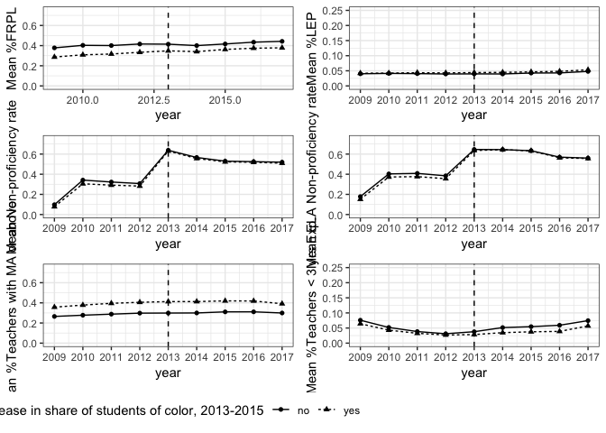
By and large, these trends between the two groups appear parallel, except in the case of the share of novice teachers. There may be some unobserved differences between the two groups related to school or teacher quality.
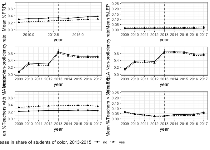
If I restrict the sample to majority white schools, the trends are parallel for all variables.
Now, turning to the difference-in-differences analysis. I will first do the vanilla regression (model 1) and then the fixed effects regression (model 2). Since it is quite likely that there is correlations within schools, it is wise to use clustered standard errors.
m1 <-
  felm(math_white_non_partic ~
         increase_blhp_2013_2015*post2013 | 0 | 0 | district_cd,
       data = ny_panel)

m2 <-
  felm(math_white_non_partic ~
         increase_blhp_2013_2015*post2013 +
         lag(math_all_students_non_prof_rate) +
         lag(math_white_non_prof_rate) +
         per_fewer_3yrs_exp +
         per_mas_plus +
         per_frpl +
         per_lep +
         log(total_enroll) | 0 | 0 | district_cd,
       data = ny_panel)

m3 <-
  felm(math_white_non_partic ~
         increase_blhp_2013_2015*post2013 | 0 | 0 | district_cd,
       data = ny_panel %>%
         filter(mean_per_white > 0.6))
m4 <-
  felm(math_white_non_partic ~
         increase_blhp_2013_2015*post2013 +
         lag(math_all_students_non_prof_rate) +
         lag(math_white_non_prof_rate) +
         per_fewer_3yrs_exp +
         per_mas_plus +
         per_frpl +
         per_lep +
         log(total_enroll) | 0 | 0 | district_cd,
       data = ny_panel %>%
         filter(mean_per_white > 0.6))

coef_names <- unique(c(names(coef(m2))))

names(coef_names) <- unique(c(names(coef(m2))))

names(coef_names)[11] <- c("Increase in %Black/Latinx, 2013-2015")

huxreg(list(`DID estimator only` = m1,
            `Full model` = m2,
            `DID estimator only` = m3,
            `Full model` = m4),
       statistics = c("N" = "nobs", "R2" = "r.squared", "Adj. R2" = "adj.r.squared"),
       coefs = coef_names[11]) %>%
  insert_row(c("", "All Schools", "", "Majority White Schools", ""), after = 0) %>%
  set_colspan(1, c(2, 4), 2) %>%
  set_top_border(1, 1:5, 0) %>%
  set_top_border(2, 1, 0) %>%
  set_top_border(3, 1:5, 1) %>%
  print_md()
| All Schools | Majority White | Schools | ||
|---|---|---|---|---|
| DID estimator only | Full model | DID estimator only | Full model | |
| Increase in %Black/Latinx, 2013-2015 | 0.065 *** | 0.065 *** | 0.056 *** | 0.056 *** |
| (0.012) | (0.011) | (0.012) | (0.011) | |
| N | 18637 | 17193 | 13638 | 12366 |
| R2 | 0.377 | 0.407 | 0.428 | 0.453 |
| Adj. R2 | 0.377 | 0.406 | 0.428 | 0.452 |
| *** p < 0.001; ** p < 0.01; * p < 0.05. |
As we can see, the interaction between increase_diverse and post2013 is significant and positive. Schools with increases in diversity has about 6 percentage points more students boycotting the test than schools without increase.
Let’s see if adding the fixed effects makes this association go away.
m1 <-
  felm(math_white_non_partic ~
         increase_blhp_2013_2015*post2013 | entity_cd + year | 0 | district_cd,
       data = ny_panel)

m2 <-
  felm(math_white_non_partic ~
         increase_blhp_2013_2015*post2013 +
         lag(math_all_students_non_prof_rate) +
         lag(math_white_non_prof_rate) +
         per_fewer_3yrs_exp +
         per_mas_plus +
         per_frpl +
         per_lep +
         log(total_enroll) | entity_cd + year | 0 | district_cd,
       data = ny_panel)

m3 <-
  felm(math_white_non_partic ~
         increase_blhp_2013_2015*post2013 | entity_cd + year | 0 | district_cd,
       data = ny_panel %>%
         filter(mean_per_white > 0.6))

m4 <-
  felm(math_white_non_partic ~
         increase_blhp_2013_2015*post2013 +
         lag(math_all_students_non_prof_rate) +
         lag(math_white_non_prof_rate) +
         per_fewer_3yrs_exp +
         per_mas_plus +
         per_frpl +
         per_lep +
         log(total_enroll) | entity_cd + year | 0 | district_cd,
       data = ny_panel %>%
         filter(mean_per_white > 0.6))

coef_names <- unique(c(names(coef(m2))))

names(coef_names) <- unique(c(names(coef(m2))))

names(coef_names)[10] <- c("Increase in %Black/Latinx, 2013-2015")

huxreg(list(`DID estimator only` = m1,
            `Full model` = m2,
            `DID estimator only` = m3,
            `Full model` = m4),
       statistics = c("N" = "nobs", "R2" = "r.squared", "Adj. R2" = "adj.r.squared"),
       coefs = coef_names[10]) %>%
  insert_row(c("", "All Schools", "", "Majority White Schools", ""), after = 0) %>%
  set_colspan(1, c(2, 4), 2) %>%
  print_md()
| All Schools | Majority White | Schools | ||
|---|---|---|---|---|
| DID estimator only | Full model | DID estimator only | Full model | |
| Increase in %Black/Latinx, 2013-2015 | 0.063 *** | 0.053 *** | 0.057 *** | 0.054 *** |
| (0.012) | (0.011) | (0.012) | (0.012) | |
| N | 18637 | 17193 | 13638 | 12366 |
| R2 | 0.709 | 0.728 | 0.752 | 0.766 |
| Adj. R2 | 0.668 | 0.685 | 0.719 | 0.731 |
| *** p < 0.001; ** p < 0.01; * p < 0.05. |
Case closed, right? Not quite. This evidence is compelling, but there is still potential bias in our results. Namely, if there are any changes within a school that are correlated with both increases in racial diversity and with testing boycotts, then the results are biased. There is something else contributing to the boycotts that is not picked up by my model. To give an exmaple, let’s say that schools make changes to curriculum and instruction that attact families of color to them but are not appealing to white families. In which case, these changes could drive both increases in diversity and increases in boycotting. Ruh roh. This is a plausible scenario, but one that I do not think is likely based on my knowledge of the research literature. Regardless, it is still plausible and I need to rule out this possibility. But how? These within-school changes are unobserved!
Well, for this to be the case, the changes in things like instruction and curriculum must logically precede the changes in racial diversity. So for schools that saw increases in diversity later on in the treatment period, say in between 2016 and 2017, these changes had to have occurred in the preceding years.
So, I will conduct a placebo test.
A placebo test
I created a new “treatment” indicator for schools that had increases in diversity from 2016 to 2017, but not between 2013 and 2015. In this case, the treatment group saw an increase after 2015, but not before. The control group saw no increase in the share of students of color after 2013. If there are any leading indicators for changes in the share of students of color in a school that are related to test boycotts, this indicator should pick them up and show a positive coefficient.
Now, I will run the same models, using the placebo indicator.
placebo1_year <-
  felm(math_white_non_partic ~
         placebo*post2013 +
         lag(math_all_students_non_prof_rate) +
         lag(math_white_non_prof_rate) +
         per_fewer_3yrs_exp +
         per_mas_plus +
         per_frpl +
         per_lep +
         log(total_enroll) | entity_cd + year | 0 | district_cd,
       data = ny_panel %>%
         filter(year < 2016))

placebo2_year <-
  felm(math_white_non_partic ~
         placebo*post2013 +
         lag(math_all_students_non_prof_rate) +
         lag(math_white_non_prof_rate) +
         per_fewer_3yrs_exp +
         per_mas_plus +
         per_frpl +
         per_lep +
         log(total_enroll) | entity_cd + year | 0 | district_cd,
       data = ny_panel %>%
         filter(year < 2016,
                mean_per_white > 0.6))

placebo_models <- list(`All Schools` = placebo1_year,
                       `Majority White Schools` = placebo2_year)

coef_names <- unique(c(names(coef(placebo1_year))))

names(coef_names) <- unique(c(names(coef(placebo1_year))))

names(coef_names)[10] <- c("Increase in %Black/Latinx, 2016-2017")

huxreg(
  placebo_models,
  coefs = coef_names[10],
  statistics = c(
    "N" = "nobs",
    "R2" = "r.squared",
    "Adj. R2" = "adj.r.squared")) %>%
  set_col_width(1,3) %>%
  set_bottom_padding(c(1:7), c(1:3), 0) %>%
  set_top_padding(c(1:7), c(1:3), 0) %>%
  print_md()
| All Schools | Majority White Schools | |
|---|---|---|
| Increase in %Black/Latinx, 2016-2017 | -0.006 | -0.012 |
| (0.009) | (0.010) | |
| N | 4030 | 2553 |
| R2 | 0.640 | 0.721 |
| Adj. R2 | 0.556 | 0.656 |
| *** p < 0.001; ** p < 0.01; * p < 0.05. |
Violà. The interaction is no longer significant, the point estimate basically zero, but not precisely estimated.